REFRACTION AT SPHERICAL SURFACES AND BY LENSES
`color{blue} ✍️` Now consider refraction at a spherical interface between two transparent media. An infinitesimal part of a spherical surface can be regarded as planar and the same laws of refraction can be applied at every point on the surface.
`color{blue} ✍️` Just as for reflection by a spherical mirror, the normal at the point of incidence is perpendicular to the tangent plane to the spherical surface at that point and, therefore, passes through its centre of curvature.
`color{blue} ✍️` We first consider refraction by a single spherical surface and follow it by thin lenses. A thin lens is a transparent optical medium bounded by two surfaces; at least one of which should be spherical.
`color{blue} ✍️` Applying the formula for image formation by a single spherical surface successively at the two surfaces of a lens, we shall obtain the lens maker’s formula and then the lens formula.
`color{brown} bbul{"Refraction at a spherical surface"}`
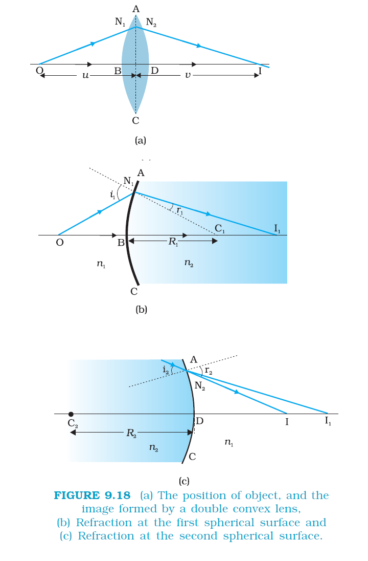
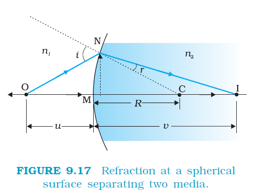
`color{blue} ✍️` Figure 9.17 shows the geometry of formation of image `I` of an object `O` on the principal axis of a spherical surface with centre of curvature `C`, and radius of curvature `R`. The rays are incident from a medium of refractive index `n_1,` to another of refractive index `n_2.`
`color{blue} ✍️` As before, we take the aperture (or the lateral size) of the surface to be small compared to other distances involved, so that small angle approximation can be made.
`color{blue} ✍️` In particular, `NM` will be taken to be nearly equal to the length of the perpendicular from the point `N` on the principal axis. We have, for small angles,
`color {purple}{tan ∠NOM = (MN)/(OM)}`
`color {purple}{tan ∠NOM = (MN)/(MC)}`
`color {purple}{tan ∠NIM = (MN)/(MI)}`
`color{blue} ✍️` Now, for `ΔNOC,` i is the exterior angle. Therefore, `i = ∠NOM + ∠NCM`
`color{blue} ✍️` Similarly, `r = angle NCM - angle NIM`
`i.e .,
`color{blue} ✍️`Now, by Snell’s law : `color{brown} {n_1 sin i = n_2 sin r}` or for small angles `color{brown} {n_1i = n_2r}`
`color{blue} ✍️` Substituting `i` and `r` from Eqs. (9.13) and (9.14), we get
`color{blue} ✍️`Here, `OM, MI` and `MC` represent magnitudes of distances. Applying the Cartesian sign convention,
`color{brown} {OM = –u, MI = +v, MC = +R}`
`color{blue} ✍️` Substituting these in Eq. (9.15), we get
`color{blue} ✍️` Equation (9.16) gives us a relation between object and image distance in terms of refractive index of the medium and the radius of curvature of the curved spherical surface. It holds for any curved spherical surface.
`color{blue} ✍️` Just as for reflection by a spherical mirror, the normal at the point of incidence is perpendicular to the tangent plane to the spherical surface at that point and, therefore, passes through its centre of curvature.
`color{blue} ✍️` We first consider refraction by a single spherical surface and follow it by thin lenses. A thin lens is a transparent optical medium bounded by two surfaces; at least one of which should be spherical.
`color{blue} ✍️` Applying the formula for image formation by a single spherical surface successively at the two surfaces of a lens, we shall obtain the lens maker’s formula and then the lens formula.
`color{brown} bbul{"Refraction at a spherical surface"}`
`color{blue} ✍️` Figure 9.17 shows the geometry of formation of image `I` of an object `O` on the principal axis of a spherical surface with centre of curvature `C`, and radius of curvature `R`. The rays are incident from a medium of refractive index `n_1,` to another of refractive index `n_2.`
`color{blue} ✍️` As before, we take the aperture (or the lateral size) of the surface to be small compared to other distances involved, so that small angle approximation can be made.
`color{blue} ✍️` In particular, `NM` will be taken to be nearly equal to the length of the perpendicular from the point `N` on the principal axis. We have, for small angles,
`color {purple}{tan ∠NOM = (MN)/(OM)}`
`color {purple}{tan ∠NOM = (MN)/(MC)}`
`color {purple}{tan ∠NIM = (MN)/(MI)}`
`color{blue} ✍️` Now, for `ΔNOC,` i is the exterior angle. Therefore, `i = ∠NOM + ∠NCM`
`color {blue}{I = (MN)/(OM) + (MN)/(MC)}`
...............(9.13)`color{blue} ✍️` Similarly, `r = angle NCM - angle NIM`
`i.e .,
`color {blue}{r = (MN)/(MC) - (MN)/(MI)}`
...........(9.14)`color{blue} ✍️`Now, by Snell’s law : `color{brown} {n_1 sin i = n_2 sin r}` or for small angles `color{brown} {n_1i = n_2r}`
`color{blue} ✍️` Substituting `i` and `r` from Eqs. (9.13) and (9.14), we get
`color {blue}{(n_1)/(OM) +n_2/(MI) = (n_2-n_1)/(MC)}`
...............(9.15)`color{blue} ✍️`Here, `OM, MI` and `MC` represent magnitudes of distances. Applying the Cartesian sign convention,
`color{brown} {OM = –u, MI = +v, MC = +R}`
`color{blue} ✍️` Substituting these in Eq. (9.15), we get
`color {blue}{(n_2)/v - (n_1)/u = (n_2-n_1)/R}`
...............(9.16)`color{blue} ✍️` Equation (9.16) gives us a relation between object and image distance in terms of refractive index of the medium and the radius of curvature of the curved spherical surface. It holds for any curved spherical surface.